Revenue model for a potential retail business selling imported products from India, based on a plan to launch one store in Bellevue, WA. Business name & idea credited to Saurabh Gangwal. March 2013.
Christopher Clayton
03/01/2013
State of the Home Furnishings Industry
The US home furnishings market grew by about 3.15% between January 2012 and January 2013 (1). Our store thus has potential to capture part of the market and become successful. It could, however, involve more risk as a niche product provider. It would also not sell furniture, a high-value product in this business category.
1. YCharts. “US Furniture and Home Furnishings Store Sales,” Census Bureau data on YCharts.com: accessed 28 February 2013. <http://ycharts.com/indicators/us_furniture_and_home_furnishings_store_sales>.
Wholesale Expenditure Regime
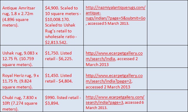
Five potential products that the retail store could sell are analyzed for realistic wholesale purchasing prices. The wholesale costs of certain samples might be used to scale retail samples to an estimated wholesale cost.
Rug/Carpet Samples
Rugs 1.1
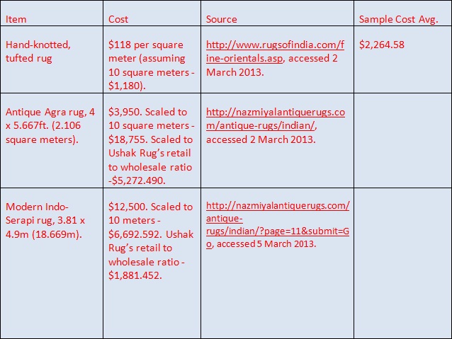
Rugs 1.2
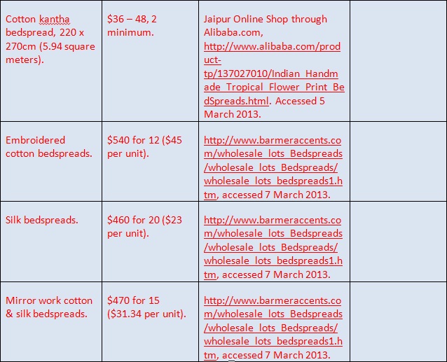
Bedspread Samples
Beadspreads 1.1
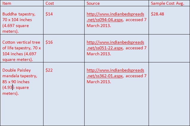
Beadspreads 1.2
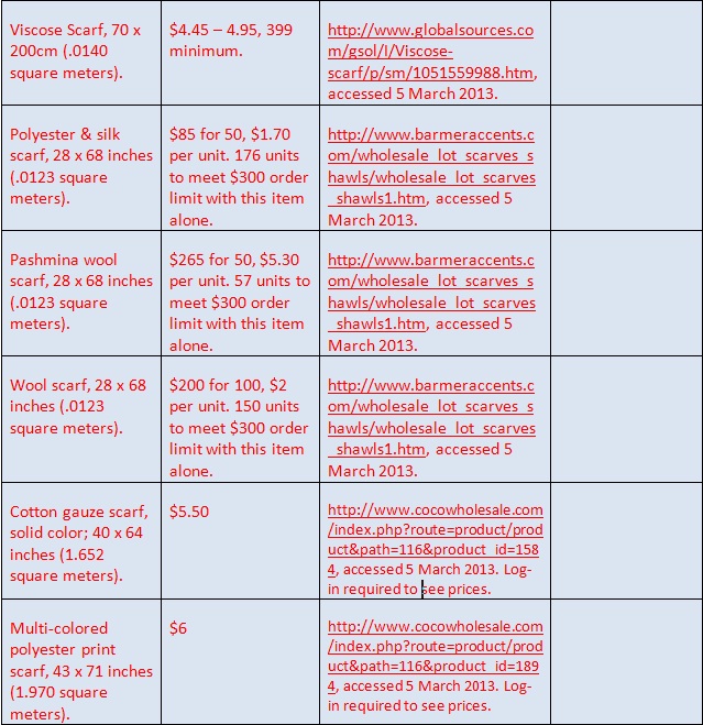
Scarf Samples
Scarves 1.1
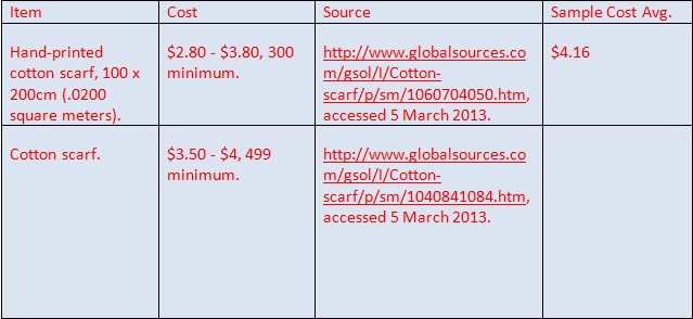
Scarves 1.2
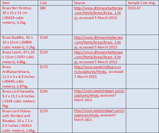
Statuette Samples
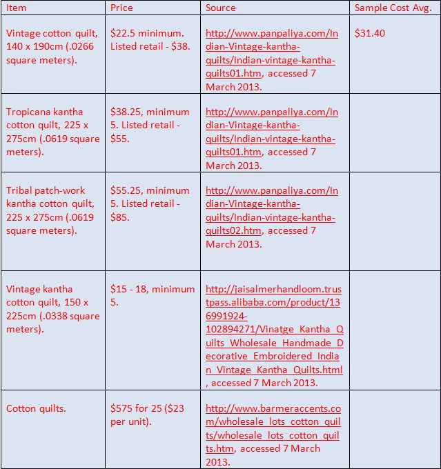
Throw/Quilt Samples
Other Costs
Other costs are predicted by category with simple averages from a sample size distributed across several sources.
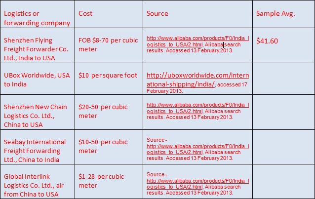
The shipping section does not reflect exact routes from a city in India to Seattle, but provides an idea of shipping costs per cubic meter in a general fashion. The maximum shipping cost provided by each company is used.
We assume that we are not hiring any employees, and take responsibility for all shop functions.
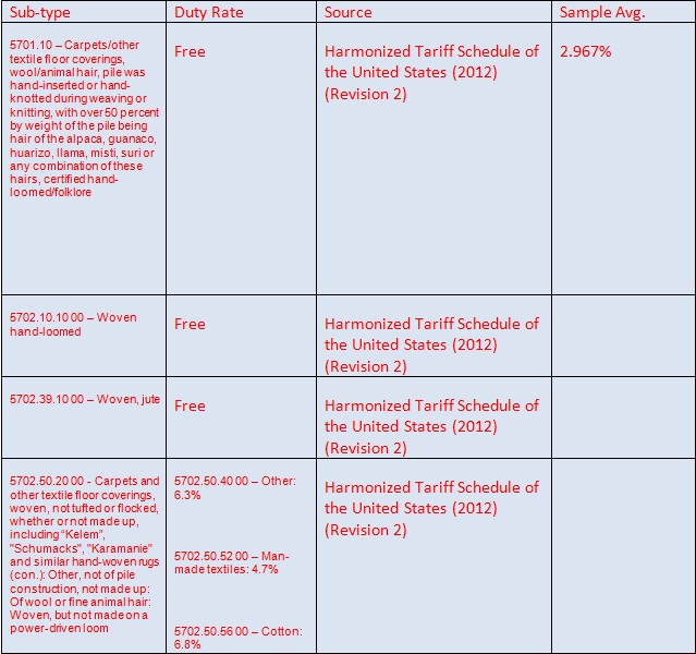
Rug/Carpet Duty Rate Samples
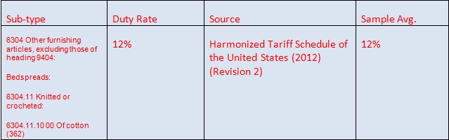
Bedspread Duty Rate Samples
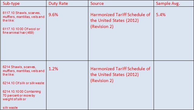
Scarf Duty Rate Samples
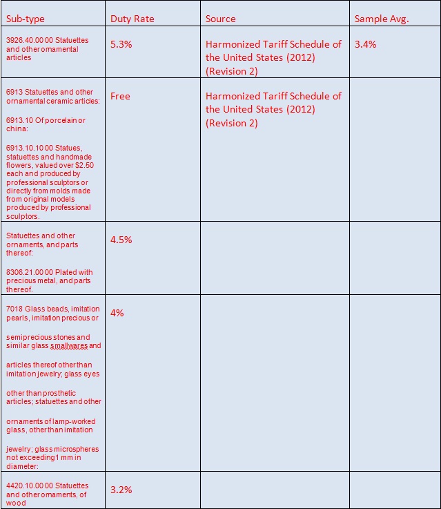
Statuette Duty Rate Samples
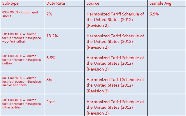
Throw/Quilt Duty Rate Samples
Shipping
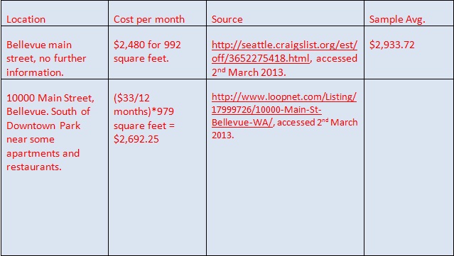
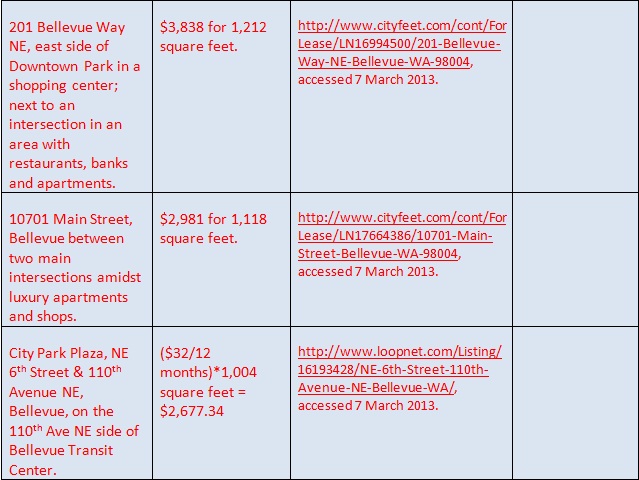
Retail Space Rent
Retail 1.1
Retail 1.2
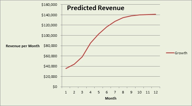
Revenue Prediction Method
For now, the product mix comes down to guessing what demand will be like, such as assuming more expensive products will not sell as highly. However, some products must be purchased in lots of minimum order quantities, and we assume the highest available statistic for this. We also assume that growth will increase after a large initial outlay of advertising spending, and then stabilize, but otherwise we are guessing at what the growth rate could be for now.
For some costs, i.e. initial IT system set-up, food and drink for the store operators (the owners) and customers, and retail racks and furniture, we are guessing at the numbers for now. Better estimates will appear under “Other Costs.”
We plan on buying 3 months’ worth of product 3 months before the store opens to serve as the initial inventory, and then 3 months’ worth at least 1 month in advance of the beginning of each subsequent 3 month period. We’ll say that supplies are renewed at the beginning of the third month in this cycle. The total quantity purchased is based on revenue growth projections and product mix out of revenue predictions. Thus the costs for these particular months sharply increase.
The break-even point is the month at which revenue and costs intersect, with different formulas used for both. The goal, however, is to break-even as quickly as possible such that the revenue curve outstrips the cost curve. We assume independent growth rates for sale quantity per item type, sale price per item type, purchase quantity per item and purchase cost per item, even if we are guessing at different growth rates right now. However, for now we can assume selling and purchasing prices will not grow but that quantity purchased and sold grows, to simplify the model.
The model follows an NPV equation, (number of products * price + number * growth rate + previous growth rate)). The beginning case does not involve any growth, and the second case does not involve previous growth. For each month, the equation for each product is added together. We take an educated guess at how many of each product might sell per month, and the growth rate for future months, with respect to all previous growth. However, it generally models logistic growth, with high growth in the beginning, until growth approaches the 2% level with relatively consistent monthly revenues. A logistic function can also do this if set up in the correct way.
The equations were solved in Mathematica, with universal variables initialized (all of the price and quantity variables), and growth variables set up before calculating each month. Dollar signs were preserved so each variable could be examined, e.g. how many numbers of each item there were for the month. Then the output was found with a calculator.
Attempts at replacing the non-formulaic, discrete and complete guess-oriented method with integration across an NPV formula with a logistic function to predict growth from initial inputs proved complicated. In particular, complicated in figuring out what the equation represented in the initial growth case, the results for month 2 (the result for month 1 is the initial revenue, on which initial growth takes place).
Predicted Revenue Formula
c(q) = carpet sale quantity
c(p) = carpet sale price
b(q) = bedspread sale quantity
b(p) = bedspread sale price
t(q) = throw/quilt sale quantity
t(p) = throw/quilt sale price
st(q) = statuette sale quantity
st(p) = statuette sale price
sc(q) = scarf sale quantity
sc(p) = scarf sale price
First month: [c(q)*c(p) + b(q)*b(p) + t(q)*t(p) + st(q)*st(p) + sc(q)*sc(p)]
Second month: [c(q)+(c(q))*(growth)*c(p)+(c(p))*(growth)] + [b(q)+(b(q))*(growth)*b(p)+(b(p)*(growth)) + [t(q)+(t(q))*(growth)*t(p)+(t(p))*(growth)] + [st(q)+(st(q))*(growth)*st(p)+(st(p))*(growth)] + (sc(q)+(sc(q))*(growth)]*sc(p)+(sc(p))*(growth)]
Third month: [c(q)+(c(q))*(growth+previous growth)*c(p)+(c(p))*(growth+previous growth)] + [b(q)+(b(q))*(growth+previous growth)*b(p)+(b(p))*(growth+previous growth)) + [t(q)+(t(q))*(growth+previous growth)*t(p)+(t(p))*(growth+previous growth)] + [st(q)+(st(q))*(growth+previous growth)*st(p)+(st(p))*(growth+previous growth)] + sc(q)+(sc(q))*(growth+previous growth)]*sc(p)+(sc(p))*(growth+previous growth)]
Etc. for each subsequent month.
Predicted Cost Formula
c(q) = Initial carpet purchase quantity
c(p) = Initial carpet purchase price
b(q) = Initial bedspread purchase quantity
b(p) = Initial bedspread purchase price
t(q) = Initial throw/quilt purchase quantity
t(p) = Initial throw/quilt purchase price
st(q) = Initial statuette purchase quantity
st(p) = Initial statuette purchase price
sc(q) = Initial scarf purchase quantity
sc(p) = Initial scarf purchase price
a(1) - a(12) = advertising costs for the month
IT = IT system creation costs
f = food and drink costs
r = retail racks and other furnishing costs
cu(c) = carpet Customs rate
cu(b) = bedspread Customs rate
cu(t) = throw/quilt Customs rate
cu(st) = statuette Customs rate
cu(sc) = scarf Customs rate
sh = shipping rate per square meter
m(c) = cubic meters per carpet
m(b) = cubic meters per bedspread
m(t) = cubic meters per throw/quilt
m(st) = cubic meters per statuette
m(sc) = cubic meters per scarf
i(0) - i(3) = purchase value of goods for a next 3 month sales period, after completing predicted revenue to have predicted sales quantities in mind for that next period.
Pre-opening: i(0)
First month: c(q)*c(p) + b(q)*b(p) + t(q)*t(p) + st(q)*st(p) + sc(q)*sc(p) + cu(c)*[c(q)*c(p)] + cu(b)*[b(q)*b(p)] + cu(t)*[t(q)*t(p)] + cu(st)*[st(q)*st(p)] + cu(sc)*[sc(q)*sc(p)] + sh*[m(c)*c(q)] + sh*[m(b)*b(q)] + sh*[m(t)*t(q)] + sh*[m(st)*st(q) + sh*[m(sc)*sc(q)] + IT + f + r + a1
Second month: [c(q)+(c(q))*(growth)*cp(p)+(c(p))*(growth)] + [b(q)+(b(q))*(growth)*b(p)+(b(p)*(growth)) + [t(q)+(t(q))*(growth)*t(p)+(t(p))*(growth)] + [st(q)+(st(q))*(growth)*st(p)+(st(p))*(growth)] + sc(q)+(sc(q))*(growth)]*sc(p)+(sc(p))*(growth)] + (cu(c)*[c(q)*c(p)] + cu(b)*[b(q)*b(p)] + cu(t)*[t(q)*t(p)] + cu(st)*[st(q)*st(p)] + cu(sc)*[sc(q)*sc(p)] + sh*[m(c)*c(q)] + sh*[m(b)*b(q)] + sh*[m(t)*t(q)] + sh*[m(st)*st(q) + sh*[m(sc)*sc(q)] + f(1+growth due to more customers) + a2
Third month: [c(q)+(c(q))*(growth+previous growth)*c(p)+(c(p))*(growth+previous growth)] + [b(q)+(b(q))*(growth + previous growth)*b(p)+(b(p)*(growth+previous growth)) + [t(q)+(t(q))*(growth+previous growth)*t(p)+(t(p))*(growth+previous growth)] + [st(q)+(st(q))*(growth+previous growth)*st(p)+(st(p))*(growth+previous growth)] + sc(q)+(sc(q))*(growth+previous growth)]*sc(p)+(sc(p))*(growth+previous growth)] + (cu(c)*[c(q)*c(p)] + cu(b)*[b(q)*b(p)] + cu(t)*[t(q)*t(p)] + cu(st)*[st(q)*st(p)] + cu(sc)*[sc(q)*sc(p)] + sh*[m(c)*c(q)] + sh*[m(b)*b(q)] + sh*[m(t)*t(q)] + sh*[m(st)*st(q) + sh*[m(sc)*sc(q)] + f(1+growth due to more customers+previous growth) + a3 + i(1)
Etc. for each subsequent month. Next round of supplies bought at the beginning of the 6th month, then the 9th month.
Sample Formula Values & Logic
We are guessing at what retail price we could sell certain products. However, for carpets, we know they could sell for about $6,000, so we will underestimate that we could sell our carpets for $4,500 each, with an average cost of carpets sold at $2,500 (overestimating) for the cost formula. We’ll assume a 3.5% duty rate, even though the carpets would most likely be duty-free. For any item we’ll assume a shipping cost of $50 per cubic meter.
For space taken up by carpets - we’ll assume a pile height of .5 inches or .0127 meters (sample - http://www.rakuten.com/pr/product.aspx?sku=218139595, accessed 2nd March 2013). Therefore the sample size’s average volume is .129 cubic meters, assuming 10 square meters per carpet.
We’ll assume a similar cost of goods sold vs. price ratio for scarves, overestimating at $33 to purchase a scarf. Therefore, we have $60 retail. Assumed average volume = (.0127 meter height) * (.0200 meters squared) = .000254 meters cubed. 9.6% duty rate because of probable non-silk composition.
Bedspreads - $30 acquisition, $54 retail, (.0127 meter height) * (5 meters squared) = .0635 meters cubed. 12% duty rate.
Throws/quilts - $35 acquisition, $63 retail. (.0127 meter height) * (.05 square meters) = .000635 cubic meters. 8% duty rate.
Statuettes - $200 acquisition, $360 retail, .0100 cubic meters. 4.5% duty rate, assuming metal composition.
We’ll assume $3,000 to set up a good server and other IT features, $5,000 in store furnishings and set-up, and $2,000 in food per month.
Revenue Prediction Given These Values
Plug in values discussed into appropriate software (e.g. Mathematica).
Prediction Table 1.1
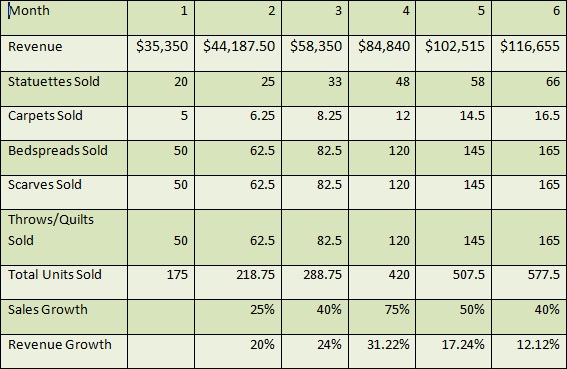
PredictionTable 1.2
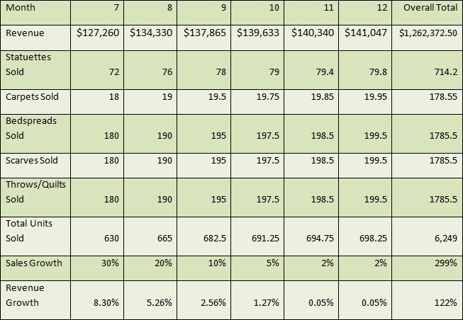
Graph